Collecting data using ArcGIS Collector

Introduction:

Although GPS allow for a high level of positional accuracy, when collecting data in the field, they are often extremely laborious when it comes to data entry. The GPS units have slow processors, and poorly responsive screens. ArcCollector is an application for smartphones that allows for expedited data entry when recording data in the field. It requires a cellphone signal, which may slightly limit its usable range, but its use of the smartphones' hardware allows for intuitive data entry.

Methods:

Before performing data collection, a geodatabase needed to be created. I recorded weather data around campus, and differentiated between points by how exposed the locations were to wind. I created four domains: a coded value domain for exposure, a range domain for temperature, a range domain for wind speed, and a range domain for wind direction. After all of the domains were created, I created a feature class, and assigned the domains to attribute fields. After the feature class was created, I customized its symbology so every exposure level had a different symbol associated with it. Next, I shared the ArcMap document to ArcGIS online so I could collect data in the field.

Performing the data collection with ArcCollector was easy. Attribute entry as performed by typing the values into a form using an on-screen keyboard. I recorded the temperature and wind speed with a Kestrel Anemometer. I used a compass to determine the direction snow was falling, in order to identify the wind direction.

Discussion:

Entering attribute data using ArcCollector was substantially easier than using the Topcon Tesla or a Trimble Juno. The positional accuracy of ArcCollector was rather low, as one of the points was located in a building.

Results:

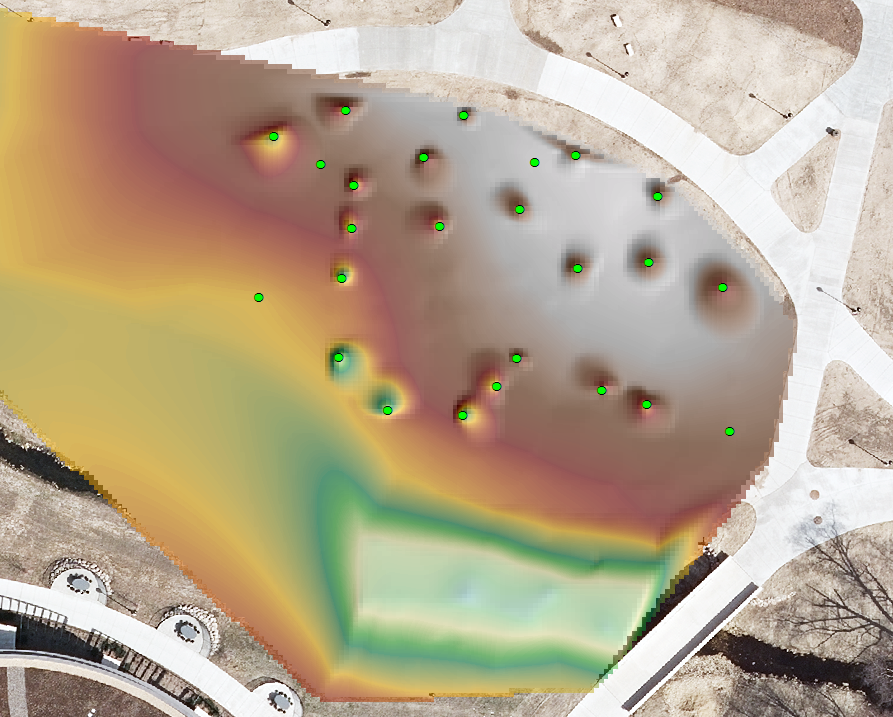
After the collection was complete, I interpolated the wind speeds and wind directions between the points using the Nearest Neighbor method. I then used the "raster domain" tool to create a polygon layer of the extent of the interpolated surfaces. Next, I used the "erase" tool with a polygon feature class of the buildings on campus to eliminate the buildings' areas from the extent feature class. The "create random points" tool was used to create 100 random points within this newly erased polygon feature class. I used the "extract multi values to points" tool to assign the wind speed and direction rasters' values to the random points. I then symbolized the points as arrows, with proportional sizes related to their wind speeds. I used an advanced option to rotate the arrows to the value extracted from the wind direction raster (Figures 1,2).

Figure 1: Mapped wind values with the collected points.

Figure 2: Wind values mapped with ArcScene, to see the interaction between wind and buildings.

Conclusion:

ArcCollector is not good at collecting points in situations where positional accuracy is important. However, it allows for extremely fast entry of attribute data, a quality that increases its desirability, specifically as the number of entered attributes per point increases.




Sources:
http://en.acolita.com/how-to-create-a-wind-map-in-arcgis.html

Terrain Survey with Dual Frequency GPS and Total Station

Introduction:

When performing a terrain survey, two major factors need to be considered: accuracy and speed. We performed terrain surveys using two different methods in order to see how each method performed according to these factors.

Study Area:

The point collections were performed in the UW - Eau Claire campus commons (Figure 1).

Figure 1: Our study area.

Methods:

The first point collection was using Real-Time-Kinematic GPS (RTK). RTK allows for extremely high positional accuracy, as it is constantly getting a correction signal via an internet connection. The internet connection was provided by a Verizon MiFi, which allowed us to collect using a corrected signal regardless of our location. The points were recorded with a Topcon Tesla, which was connected to a Topcon Hiper SR. When we collected points, we had the receiver collect 10 positional points at every collected location.

Figure 2: Casey using RTK to record the "backsite" point while David shivers while holding the prism rod. 

The second point collection method was Total Station. Total Station works as an advanced form of distance azimuth survey. If the distance and azimuth between a known point and another location is recorded, it is possible to determine the location and elevation of the location. First, two points needed to be collected using RTK, with one of the points where we were to set up the total station ("occupied point"), and the second point ("backsite point") at another location. Next, we set up the total station over the first point, so the center of the tripod was over the collected point's location. After the tripod was in the proper location, it needed to be leveled, so the points would all be collected accurately. After the total station was leveled, we fired the laser at the second RTK point in order to calibrate the total station's azimuth and distance readings. This is called "shooting the backsite". After the system is calibrated, points were recorded by having a person hold the prism rod while a second person fires a laser into the center of the prism. The distance and azimuth recordings from the laser were recorded by the Topcon Tesla.


Results:

When the positions of all 10 points were averaged, the RTK had horizontal accuracy of ~3mm and vertical accuracy of ~4mm. The RTK rig needed to be leveled before every point could be collected, greatly slowing the collection process.

Using Total Station to conduct a survey was slightly slower, because of the time required to set up the tripod and level the sensor. However, once these were done, it was possible to record points substantially quicker than with RTK, as there were no limitations as a result of poor GPS fixes.

The surfaces generated from the points provided a good representation of the natural environment, and didn't have any outlying points (Figure 3).

Figure 3: Points collected with RTK are symbolized in green,
and points collected with Total Station are symbolized in blue.

One of the other groups' total station points sustained some form of error, and caused a pock-marked texture across the surface (Figure 4).

Figure 4: The inaccurate points are symbolized in bright green.

Conclusions:

Both methods allow for accurate data to be collected, and will be very useful for conducting future terrain surveys. I will probably use RTK when collecting GCPs and other highly accurate points at lower spatial densities. Total Station will be used when collecting points at higher spatial densities, as it allows data to be collected at a much higher pace.

Navigation with Map and Compass

Introduction:

In this activity, we navigated between a series of points using a map and a compass. In order to do so, we were divided into groups of three, in order to fill three different roles: Pace Counter, Azimuth Control, and Leap Frogger. The Pace Counter walks between points, counting their paces to establish distance. The Azimuth Control stands at a point, ensuring the pace counter is staying in line with the azimuth, and telling the Pace Counter which landmarks to walk towards. The Leap Frogger moves to a given landmark to allow the pace counter to move ahead, allowing the Pace Counter to better see where they are headed and the Azimuth Control to move to the Leap Frogger's previous position.

Study Area:

The Priory is a facility owned by the University of Wisconsin - Eau Claire. It is an old Benedictine Convent, surrounded by 100+ acres of forest. Conditions were overcast, and it started to get dark under the canopy about halfway through the navigation exercise.

Figure : We conducted the survey on an overcast fall day.
Temperatures were in the mid 50's which was perfect for the exercise.

Methods:

Each group was given a list of point coordinates in UTM, and told to plot the point locations on their reference map.

Figure : Marking the lines between the plotted points.

Once we had plotted our points, we drew lines between the points and determined the bearing of the lines. In order to do this we oriented our maps with magnetic north, then rotated the compass bezel so the north arrow was still in the "shed" and the heading arrow matched our line. The bearing was the point on the bezel that lined up with the heading arrow.

Figure : Marking the bearing of the lines using the compass.

Figure  : Marked Point Locations on Map.

When marking our points we realized that the first point was directly on one of the trails, so we decided to walk along the trail in order to get to our first point. After we got to the point, we realized we had never recorded our distances, so we marked the end points of the bearing lines on the edge of a piece of paper, and measured the distance with an app on David's phone. After getting the linear distance, we converted the distances to paces, using my pace count of 64 paces / 100 meters. After writing down the pace counts for all of the bearing lines, we started navigating with myself as the Pace Counter, David as Azimuth Control, and Aly as Leapfrogger. Unfortunately, we didn't understand what the leapfrogger was suppposed to do, so Aly essentially just leaped to my position after I had paced it out, and made sure that it matched David's Azimuth.

Figure : Myself counting paces between point one and our first leapfrog point.

The area between the first and second points was densely vegetated, so we were only able to travel short distances between leaps. We ended up being fairly certain we were on the right bearing, but the full pace count left me around 10 meters short of our objective. This was likely due to the substantial obstacles I had to navigate over, including but not limited to: downed trees, remnants of an old garage, steep ravine slopes, and a 10 meter wide patch of stinging nettles. As there was actually no marker at location two, our accuracy estimate is truly only an estimate.

Figure : The woman in blue is standing where we estimated the second point to be.
I was standing where I had reached the full extent of the pace count,
an estimated 10 meters short of the objective.

The area between points two and three was primarily a jack pine forest with little to no underbrush, which made navigating a breeze. I was slightly more comfortable with my pace count, and our resulting location was still short of our objective point.

Figure : The man on the left side of the image is standing next to point three,
while I am standing where I had reached the full extent of the pace count.

This time, however, we realized that our azimuth was the major cause of error.

Figure : The Line-Of-Sight graph shows visibility from point two.
After reaching the top of the ravine, we calculated our bearing incorrectly, and we ended up at an incorrect location. 

After reaching point three, we had David and Aly switch roles.

Figure : Aly determining a landmark according to the azimuth from point three.

As we were again navigating the jack pine forest, the pace count gave us a very accurate sense of distance. We navigated the bearing in three leaps, each of which was unfortunately moving on the wrong azimuth.

Figure : If we had followed the field calculations correctly, we would have ended at the pink dot near point 4.
The tracklog points show that our azimuth very clearly deviated from that calculated heading.

Our navigation between points four and five was perfectly accurate to the point marked on the map. Points four and five were close enough together that no leaping was necessary in order to navigate between them. This certainly aided the accuracy of navigation.

Figure : The Line-Of-Sight tool shows point five was within sight from point four.

Discussion:

Our reference maps should've also had intermediate reference lines at 25 meter increments in addition to the 50 meter increments we used. Smaller increments would've allowed easier plotting of the points.

We experienced error from a number of different sources. Our navigation between points one to two, and points three to four was negatively impacted by poor azimuth readings. Our field calculated azimuths were fairly accurate, but our navigation wasn't leading to the conclusion of incorrect azimuth readings.

Sources:
https://web.viu.ca/corrin/FRST121/Help/UTM%20Coordinates.pdf