Introduction:
We were tasked to create a landscape within a 1.26m x 1.19m wooden frame featuring: a plain, a mountain, a ridge, a valley, and a depression.
After forming our landscape, we were to survey the surface of the landscape for
future mapping purposes. We were to form our landscape on the sandy point bar
of the Chippewa River underneath the UW-EC campus footbridge.
Methods:
Before shaping the terrain, we leveled the ground surface
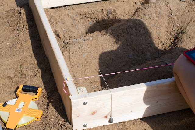
underneath the survey frame, in order to standardize the elevations for our survey. After the frame was leveled, we created a hill along the left side of the frame, a valley running from the top left to the bottom right, a ridge running parallel to the valley, a depression in the top right corner, and a plain in the lower left corner (Figures 4-5). Next, we put scotch tape over the edges of the frame and marked them with a pen at 10cm
intervals from a point of origin on the inside edge of “1D” on the frame (Figures 1-3). The
boards themselves were all the same length, but due to the frame’s design, the X-axis
(from 1D to 1B) was 1.26m long, and the Y-axis (from 1D to 1C) was 1.19m long. We
made a grid with a sampling interval of 1dm, making a 12 x 11 grid with 132
total points. We started our survey at (1,1) which we found by placing
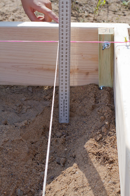
modifiable string gridlines 10cm from the origin point of the X and Y-axes. After the gridlines were in
place and pulled taut, we recorded the distance from the gridlines to the
ground surface using a meter stick and recorded them in centimeters to 1mm
accuracy (Figures 6-8). We recorded the distances from the grid to the ground as Z-values in
a Google drive spreadsheet. After scanning point (1,1,19.8), we scanned (1,2,19.8) and
continued working our way up the Y-axis until reaching the top of the frame, at
which point we moved to (2,1,19.3) and followed the same procedure. We continued in
this fashion until the survey was completed. We decided to use the base of the
boards as our sea level. The boards of the frame measured 18.1cm tall, so I
created a calculated column in Excel to subtract the distance between the
gridline and the ground from the frame height. This made a new column with the
height above or below sea level.
Discussion/Conclusion:
Leveling the frame was incredibly helpful, as it allowed us
to record the actual slope of the pre-existing plain, and the landscape as a
whole. Choosing the base of the frame as “sea level” wasn’t the best practice
as most of the plain and other features are below “sea level”. Measuring the
distance below the gridlines allowed most areas to be measured with ease, as
none of our features surpassed the frame height. The only area that caused
difficulties was the middle of the frame between (5,5) and (8,7), as they
caused a lot of movement in the arm of our ruler holder as he was surpassing
the comfortable range of his reach. This area was also more difficult to survey
because the distance from the ruler caused some issues with properly sighting
the distances between the ruler and the gridlines. Upon conducting a little
research into sampling methods, I learned that my group conducted our survey
using “systematic sampling” and that this sampling method may have caused us to
under-sample some areas and features that fell between the gridlines. To
compensate for this under-sampling, we should have instead used the “stratified
random sampling” method. In order to have used “stratified random sampling” we
would have created a grid system, and sampled one random point from within each
individual square of the grid, rather than just from their verticies.
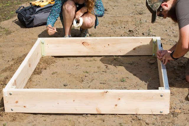 |
| Figure 1. Marking the X and Y axes on the leveled frame |
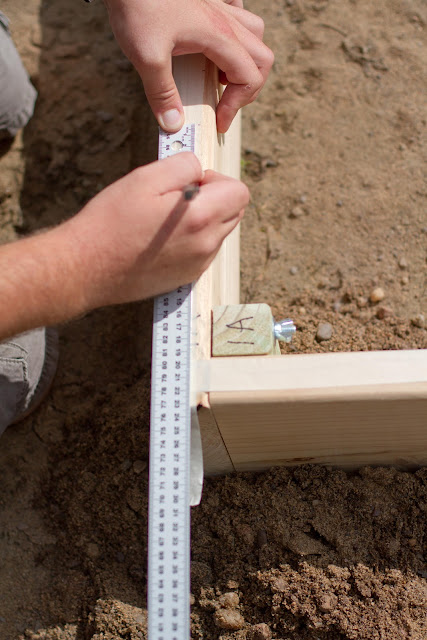 |
| Figure 2. Ensuring we have accurate measurements |
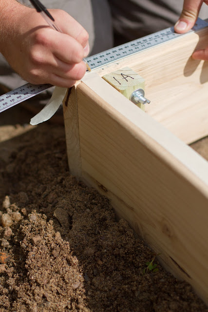 |
| Figure 3. |
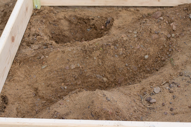 |
| Figure 4. The origin point is in the lower right corner of this photograph. |
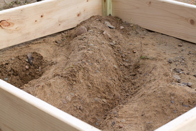 |
Figure 5. The origin point is in the bottom of the frame.
Clockwise from the left: Depression, Ridge, Plain, Hill, and Valley |
 |
| Figure 6. The grid set up to record (1,10) the origin is to the right. |
 |
| Figure 7. Recording point (1, 10, 22.9) |
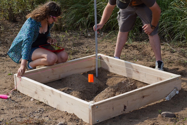 |
| Figure 8. Conducting the survey. |
Sources: http://uts.cc.utexas.edu/~wd/courses/373F/notes/lec15sam.html


No comments:
Post a Comment