Collecting data using ArcGIS Collector

Introduction:

Although GPS allow for a high level of positional accuracy, when collecting data in the field, they are often extremely laborious when it comes to data entry. The GPS units have slow processors, and poorly responsive screens. ArcCollector is an application for smartphones that allows for expedited data entry when recording data in the field. It requires a cellphone signal, which may slightly limit its usable range, but its use of the smartphones' hardware allows for intuitive data entry.

Methods:

Before performing data collection, a geodatabase needed to be created. I recorded weather data around campus, and differentiated between points by how exposed the locations were to wind. I created four domains: a coded value domain for exposure, a range domain for temperature, a range domain for wind speed, and a range domain for wind direction. After all of the domains were created, I created a feature class, and assigned the domains to attribute fields. After the feature class was created, I customized its symbology so every exposure level had a different symbol associated with it. Next, I shared the ArcMap document to ArcGIS online so I could collect data in the field.

Performing the data collection with ArcCollector was easy. Attribute entry as performed by typing the values into a form using an on-screen keyboard. I recorded the temperature and wind speed with a Kestrel Anemometer. I used a compass to determine the direction snow was falling, in order to identify the wind direction.

Discussion:

Entering attribute data using ArcCollector was substantially easier than using the Topcon Tesla or a Trimble Juno. The positional accuracy of ArcCollector was rather low, as one of the points was located in a building.

Results:

After the collection was complete, I interpolated the wind speeds and wind directions between the points using the Nearest Neighbor method. I then used the "raster domain" tool to create a polygon layer of the extent of the interpolated surfaces. Next, I used the "erase" tool with a polygon feature class of the buildings on campus to eliminate the buildings' areas from the extent feature class. The "create random points" tool was used to create 100 random points within this newly erased polygon feature class. I used the "extract multi values to points" tool to assign the wind speed and direction rasters' values to the random points. I then symbolized the points as arrows, with proportional sizes related to their wind speeds. I used an advanced option to rotate the arrows to the value extracted from the wind direction raster (Figures 1,2).

Figure 1: Mapped wind values with the collected points.

Figure 2: Wind values mapped with ArcScene, to see the interaction between wind and buildings.

Conclusion:

ArcCollector is not good at collecting points in situations where positional accuracy is important. However, it allows for extremely fast entry of attribute data, a quality that increases its desirability, specifically as the number of entered attributes per point increases.




Sources:
http://en.acolita.com/how-to-create-a-wind-map-in-arcgis.html

Terrain Survey with Dual Frequency GPS and Total Station

Introduction:

When performing a terrain survey, two major factors need to be considered: accuracy and speed. We performed terrain surveys using two different methods in order to see how each method performed according to these factors.

Study Area:

The point collections were performed in the UW - Eau Claire campus commons (Figure 1).

Figure 1: Our study area.

Methods:

The first point collection was using Real-Time-Kinematic GPS (RTK). RTK allows for extremely high positional accuracy, as it is constantly getting a correction signal via an internet connection. The internet connection was provided by a Verizon MiFi, which allowed us to collect using a corrected signal regardless of our location. The points were recorded with a Topcon Tesla, which was connected to a Topcon Hiper SR. When we collected points, we had the receiver collect 10 positional points at every collected location.

Figure 2: Casey using RTK to record the "backsite" point while David shivers while holding the prism rod. 

The second point collection method was Total Station. Total Station works as an advanced form of distance azimuth survey. If the distance and azimuth between a known point and another location is recorded, it is possible to determine the location and elevation of the location. First, two points needed to be collected using RTK, with one of the points where we were to set up the total station ("occupied point"), and the second point ("backsite point") at another location. Next, we set up the total station over the first point, so the center of the tripod was over the collected point's location. After the tripod was in the proper location, it needed to be leveled, so the points would all be collected accurately. After the total station was leveled, we fired the laser at the second RTK point in order to calibrate the total station's azimuth and distance readings. This is called "shooting the backsite". After the system is calibrated, points were recorded by having a person hold the prism rod while a second person fires a laser into the center of the prism. The distance and azimuth recordings from the laser were recorded by the Topcon Tesla.


Results:

When the positions of all 10 points were averaged, the RTK had horizontal accuracy of ~3mm and vertical accuracy of ~4mm. The RTK rig needed to be leveled before every point could be collected, greatly slowing the collection process.

Using Total Station to conduct a survey was slightly slower, because of the time required to set up the tripod and level the sensor. However, once these were done, it was possible to record points substantially quicker than with RTK, as there were no limitations as a result of poor GPS fixes.

The surfaces generated from the points provided a good representation of the natural environment, and didn't have any outlying points (Figure 3).

Figure 3: Points collected with RTK are symbolized in green,
and points collected with Total Station are symbolized in blue.

One of the other groups' total station points sustained some form of error, and caused a pock-marked texture across the surface (Figure 4).

Figure 4: The inaccurate points are symbolized in bright green.

Conclusions:

Both methods allow for accurate data to be collected, and will be very useful for conducting future terrain surveys. I will probably use RTK when collecting GCPs and other highly accurate points at lower spatial densities. Total Station will be used when collecting points at higher spatial densities, as it allows data to be collected at a much higher pace.

Navigation with Map and Compass

Introduction:

In this activity, we navigated between a series of points using a map and a compass. In order to do so, we were divided into groups of three, in order to fill three different roles: Pace Counter, Azimuth Control, and Leap Frogger. The Pace Counter walks between points, counting their paces to establish distance. The Azimuth Control stands at a point, ensuring the pace counter is staying in line with the azimuth, and telling the Pace Counter which landmarks to walk towards. The Leap Frogger moves to a given landmark to allow the pace counter to move ahead, allowing the Pace Counter to better see where they are headed and the Azimuth Control to move to the Leap Frogger's previous position.

Study Area:

The Priory is a facility owned by the University of Wisconsin - Eau Claire. It is an old Benedictine Convent, surrounded by 100+ acres of forest. Conditions were overcast, and it started to get dark under the canopy about halfway through the navigation exercise.

Figure : We conducted the survey on an overcast fall day.
Temperatures were in the mid 50's which was perfect for the exercise.

Methods:

Each group was given a list of point coordinates in UTM, and told to plot the point locations on their reference map.

Figure : Marking the lines between the plotted points.

Once we had plotted our points, we drew lines between the points and determined the bearing of the lines. In order to do this we oriented our maps with magnetic north, then rotated the compass bezel so the north arrow was still in the "shed" and the heading arrow matched our line. The bearing was the point on the bezel that lined up with the heading arrow.

Figure : Marking the bearing of the lines using the compass.

Figure  : Marked Point Locations on Map.

When marking our points we realized that the first point was directly on one of the trails, so we decided to walk along the trail in order to get to our first point. After we got to the point, we realized we had never recorded our distances, so we marked the end points of the bearing lines on the edge of a piece of paper, and measured the distance with an app on David's phone. After getting the linear distance, we converted the distances to paces, using my pace count of 64 paces / 100 meters. After writing down the pace counts for all of the bearing lines, we started navigating with myself as the Pace Counter, David as Azimuth Control, and Aly as Leapfrogger. Unfortunately, we didn't understand what the leapfrogger was suppposed to do, so Aly essentially just leaped to my position after I had paced it out, and made sure that it matched David's Azimuth.

Figure : Myself counting paces between point one and our first leapfrog point.

The area between the first and second points was densely vegetated, so we were only able to travel short distances between leaps. We ended up being fairly certain we were on the right bearing, but the full pace count left me around 10 meters short of our objective. This was likely due to the substantial obstacles I had to navigate over, including but not limited to: downed trees, remnants of an old garage, steep ravine slopes, and a 10 meter wide patch of stinging nettles. As there was actually no marker at location two, our accuracy estimate is truly only an estimate.

Figure : The woman in blue is standing where we estimated the second point to be.
I was standing where I had reached the full extent of the pace count,
an estimated 10 meters short of the objective.

The area between points two and three was primarily a jack pine forest with little to no underbrush, which made navigating a breeze. I was slightly more comfortable with my pace count, and our resulting location was still short of our objective point.

Figure : The man on the left side of the image is standing next to point three,
while I am standing where I had reached the full extent of the pace count.

This time, however, we realized that our azimuth was the major cause of error.

Figure : The Line-Of-Sight graph shows visibility from point two.
After reaching the top of the ravine, we calculated our bearing incorrectly, and we ended up at an incorrect location. 

After reaching point three, we had David and Aly switch roles.

Figure : Aly determining a landmark according to the azimuth from point three.

As we were again navigating the jack pine forest, the pace count gave us a very accurate sense of distance. We navigated the bearing in three leaps, each of which was unfortunately moving on the wrong azimuth.

Figure : If we had followed the field calculations correctly, we would have ended at the pink dot near point 4.
The tracklog points show that our azimuth very clearly deviated from that calculated heading.

Our navigation between points four and five was perfectly accurate to the point marked on the map. Points four and five were close enough together that no leaping was necessary in order to navigate between them. This certainly aided the accuracy of navigation.

Figure : The Line-Of-Sight tool shows point five was within sight from point four.

Discussion:

Our reference maps should've also had intermediate reference lines at 25 meter increments in addition to the 50 meter increments we used. Smaller increments would've allowed easier plotting of the points.

We experienced error from a number of different sources. Our navigation between points one to two, and points three to four was negatively impacted by poor azimuth readings. Our field calculated azimuths were fairly accurate, but our navigation wasn't leading to the conclusion of incorrect azimuth readings.

Sources:
https://web.viu.ca/corrin/FRST121/Help/UTM%20Coordinates.pdf

Navigation Map Construction

Introduction:

The purpose of this exercise was for us to create maps to be used in navigation activities in the future. We created two maps, one with the World Geodetic Survey 1984 (WGS84) coordinate system, and one with the Universal Transverse Mercator (UTM) coordinate system.

Methods:

We needed to create a map using each coordinate system, with grid lines that were appropriate for the respective systems. I generated elevation rasters and contour lines from LiDAR the city acquired in 2013. I also added maps of the trails that I had previously collected with a Trimble Juno 3b when conducting research. I think the trails will be a good reference for knowing how far past or before  trail the markers are. I used 10ft contours, as they would show the terrain better than a 5 meter contour, but be less distracting than the 2ft contours my professor offered. I refrained from adding an aerial image, as I have a fair understanding of the Priory's landscape and I didn't think the map needed any additional clutter. After designing the maps, I added both my and one of my partner's pace counts, so we would have them recorded for reference in the field.

Figure 1: The UTM zones for the lower 48 U.S. States.
I used UTM zone 15N to create my reference map.

Universal Transverse Mercator breaks the whole planet into 60 different zones that are 6 degrees wide, which reduces overall distortion of the areas within the grid. Locations are measured as "northings" and "eastings", or distances from the equator and from a false origin. The central meridian of each zone is given an easting of 500,000, so all values are within the zone have a positive easting value.

Figure 2: My UTM based reference map

The World Geodetic Coordinate System 1984 (WGS84), provides coordinates as their locations on Earth's ellipsoid surface. It is used by GPS for locating positions anywhere on earth's surface and for creating extremely large scale maps.

Figure 3: My WGS84 based reference map

Discussion:

The UTM map will be extremely helpful when navigating with the compass and pace counts, as all distances on the map will be calculable in meters.

The WGS84 map won't be very helpful for navigation with the compass and pace counts, as the grid has .00056 degree intervals, which translates to 44.0776 meters. This awkward interval will make any sort of distance calculations difficult when in the field. The map will, however,  be extremely useful for the GPS navigation activity, as all of the coordinate locations will be easily identifiable on the map.

Conclusion: 

I am intrigued to see how well or poorly my navigation maps actually perform when in the field. I am expecting the trails data to be a helpful reference, though they may prove to be an unnecessary distraction.


Sources:

http://pubs.usgs.gov/fs/2001/0077/report.pdf

I used this page to convert the distances from decimal degrees to meters: https://en.wikipedia.org/wiki/Decimal_degrees

Unmanned Aerial Systems

Introduction:

What is an Unmanned Aerial System (UAS)? According to the FAA, "A UAS is the unmanned aircraft (UA) and all of the associated support equipment, control station, data links, telemetry, communications and navigation equipment, etc., necessary to operate the unmanned aircraft." A UAS differs from a remote control (RC) vehicle, in that it is operates along a preplanned course without being directly controlled by the operator.

Methods:

Part 1: Demonstration Flight

Figure 1: The DJI Phantom.

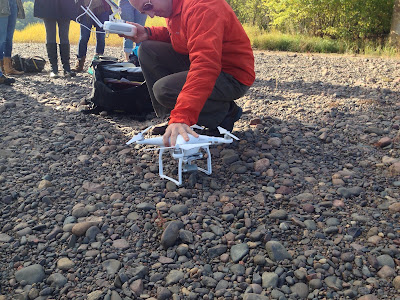
In order to introduce our class to major concepts and capabilities of UAS, our professor manually flew a DJI Phantom and captured aerial images under the university's footbridge. He selected this flight location, because there was a lot of open vertical space, and it wouldn't draw too much attention. Although it was technically being flown manually, the Phantom was fairly autonomous, hovering in position even when the operator completely removed their hands from the remote.

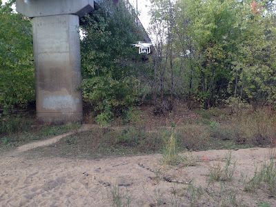
Figure 2: The Phantom in flight.

The Phantom had a camera connected via a 2 axis gimbal. The gimbal is an adjustable arm, which allows the camera to be rotated/stabilized both vertically and horizontally. The gimbal also allows the camera to be adjusted to capture images off and on nadir (from directly above).

Part 2: Software

After the demonstration flight was completed, we returned to the lab to learn how to process imagery, generate flight plans used to fly automated missions, and gain better understanding of how different types of aerial vehicles operate.

Mission Planner:
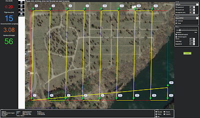
Using the software "Mission Planner", I designed a flight plan based on the following scenario: "The City of Eau Claire would like to know how many tombstones Lakeview Cemetery contains, and wants to use UAS to find out. What camera should you use, and at what altitude should you fly?".

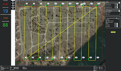
Figure 3: Flight plan using the Canon SX230 HS, flying at 98m.

Figure 4: Flight plan using the Canon 5d Mark II, flying at 98m.

I generated two separate flight plans for the same area, using different Canon camera sensors. The flight using the SX230 HS required 11 passes at 98m altitude to cover the whole area with 3.02 cm/pixel spatial resolution, for a total of 88 images. The flight using the 5d Mark II required just over 8 passes at 28m altitude to cover the whole area with 3.08cm/pixel spatial resolution, for a total of 56 images. The SX230 HS would require 19 minute flight time, and the 5d Mark II would only require a 15 minute flight time. The SX230 HS has a 12.1 megapixel sensor, and the 5d Mark II has a 21.1 megapixel sensor.

The 5d Mark II would seem like the natural choice, as it provides better quality in less time, however the devil is in the details. The the Canon SX230 HS weighs 223g and has an MSRP of $350. The camera body alone of the Canon 5d Mark II weighs 810g, a comparable lens (Canon EF 24mm 2.8 IS) weighs 280g, for a combined weight of 1,090g and with a combined cost of $1,800. These higher weights would require a UAV with a higher payload capacity, further increasing the cost.

Real Flight Flight Simulator:

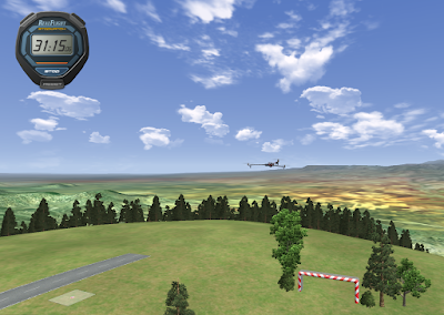
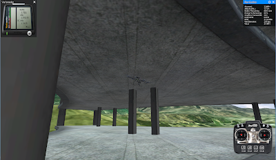
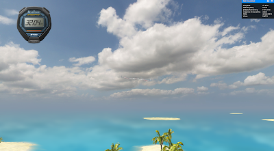
Using the software "RealFlight 7.5" I gained experience flying both fixed-wing and multi rotor aircraft. I flew two different multi rotors: the Octocopter 1000 and the Tricopter 9000. The tricopter was extremely unstable, but very fast. The octocopter was very stable, and had an attached gimbal which allowed the adjustment of an attached DSLR camera mounted on the bottom of the craft. The tricopter did not perform well in situations where micro adjustments were needed, and it crashed often when attempting to navigate through tight locations like the obstacle course (Figure 5). The octocopter, while slower, responded extremely well to micro adjustments, and handled the obstacle course and the construction site with ease (Figure 6). The octocopter also performed extremely well in high-wind conditions (Figure 7).

Figure 5: The tricopter in flight.

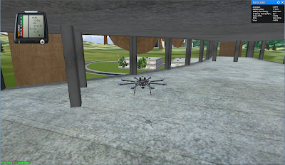
Figure 6: Navigating the octocopter through the tight spaces of a construction site.

Figure 7: The octocopter was stable even with a 15mph crosswind.

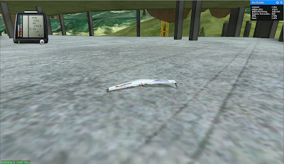
Next, I flew two fixed wing aircraft: a flying-wing called the 'Slinger', and a Vertical Take-off and Landing (VTOL) jet called the 'Harrier'. The slinger could operate at substantially higher speeds than either of the multi rotors previously tested, but was substantially more difficult to fly (Figure 8). It required higher speeds to maintain flight, and as a result, had difficulties trying to navigate the tight spaces in which the octocopter was comfortable (Figure 9). The slinger also required long horizontal distances to take off, unlike the the multi rotors. The slinger performed the best when tight spaces weren't an issue, and when it could take advantage of its greater speed.

Figure 8: The slinger in flight.

Figure 9: The result of trying to navigate the construction site in Figure 8 with the slinger.

The Harrier was a strange hybrid between the slinger and the multi rotors, as a result of its VTOL capabilities. If its turbines were directed towards the ground it could hover, and yet sustain flight at high speeds with the turbines directed directly behind it (Figure 10). It was the fastest of any of the aircraft flown, and required the longest turning distances when in full flight mode. It had the most difficulties with tight spaces because of its incredibly high speed.

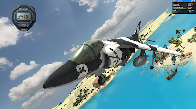
Figure 10: The harrier's turbines are visible to the left
of the bomb-shaped capsule under its wing.

Pix4D: 

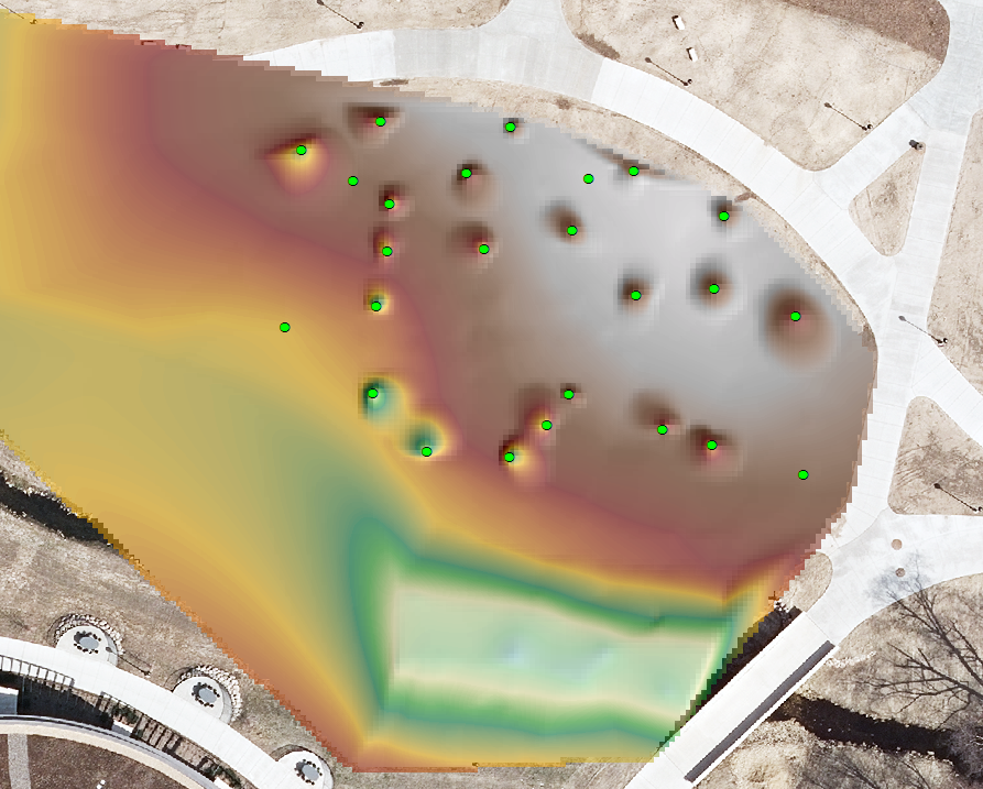
Pix4D was used to process imagery collected by the flight described in Part 1. The software analyzed the photographs, generated a point cloud, and created a DSM and Orthomosaic.

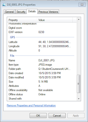
Figure 11: The DJI Phantom's images contained GPS data
Pix4D used this data to stich the images together and generate
a point cloud, DSM, and an orthomosaic

The point cloud could be used to add additional points to locations where existing LiDAR data has gaps, or generate extremely high-resolution TINs (Figure 12). The point cloud had extremely high point density of 0.007m (or .276in) (Figure 13). For comparison, the LiDAR point cloud the city obtained in 2013 for the same area has a point density of 0.45m (or 17.724in) (Figure 14).

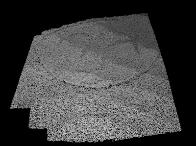
Figure 12: The generated point cloud.

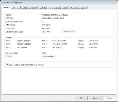
Figure 13: Properties for the LasDataset created from the Phantom data.

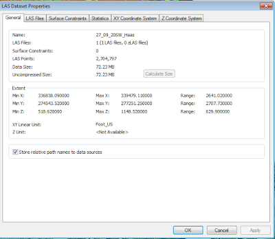
Figure 14: Properties for the Las Dataset from the Citywide LiDAR survey.

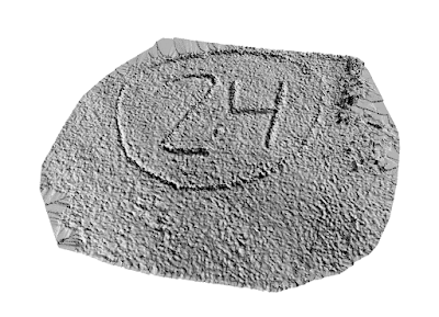
The DSM recorded subtle changed in topography extremely well, and has extremely small pixel sizes, allowing identification of individual rocks (Figure 16).

Figure 12: A hillshade created from the DSM, to show the topography.

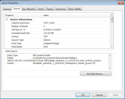
Figure 16: The DSM and Ortho have the same incredibly small pixel size of 0.00204m
This equates to 2.04mm or 0.08in.
In 2013, the City obtained aerial imagery with pixel sizes of 3in

The Orthomosaic allows for 3D models of the landscape to be created. It was created along with the DSM, so it matches perfectly with the DSM when viewed in 3D viewers, like ArcScene. The orthomosaic has 37.3 TIMES higher resolution than the existing aerial images the city obtained in 2013 (Figure 16).

Discussion:

UAS Scenario:

"A mining company wants to get a better idea of the volume they remove each week. They don’t have the money for LiDAR, but want to engage in 3D analysis"

LiDAR may be the to-go buzzword for many in the industry these days, but UAS is the way of the future. UAV photogrammetry can obtain be used to calculate volumetrics with only 0.1% error when compared to LiDAR, and for a fraction of the price. I have prepared two example scenarios for you to help determine which type of vehicle will best suit your needs.

For performing volumetrics before and after blasting, we would suggest using a 3DR X8-M. The X8-M is a multirotor aircraft with: vertical takeoff and landing capabilities, an imaging speed of 8 m/sec, and great navigability in tight spaces. The only negative of this platform is its maximum flight time of 14 minutes, necessitating additional batteries if larger survey areas are desired.

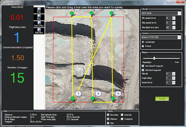
Figure 17: Flying a small wall prior to blasting with the 3DR X8-M could be done in 1 minute,
with 1.5cm/pixel ground resolution.

 For flying larger open-pit mines, or strip mines, we would suggest using the 3DR Aero-M. The Aero-M is a fixed wing platform with an imaging speed of 23m/sec and a maximum flight time of 40 minutes. The negatives of this platform are: it requires a longer turn radius at the end of each flight line - lengthening the overall length of the flight, it requires clear runways for takeoff and landing, and this platform does not perform well in tight spaces.

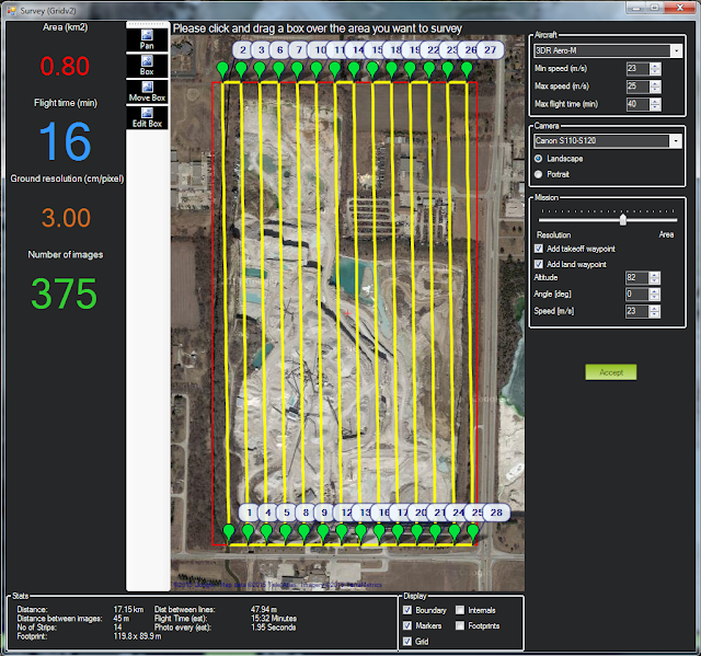
Figure 18: Flying a 0.8 km2 area with the 3DR Aero-M can be done in 16 minutes,
with 3.00cm/pixel ground resolution. 

If you are looking to map extremely long strip mines, we would suggest using the 3DR Aero-M. In every other situation, the 3DR X8-M will be the best platform.

After recording imagery, we will process it using Pix4D to create point clouds which will allow for the calculation of volumetric information. Your company will be able to know exactly how much material was moved by each blast, know the volume of your tailings piles, and know exactly how much the piles are growing each month. If you would like more information about how accurate UAV photogrammetry is when compared to LiDAR, click here.

More information can be found at the following links:
https://pix4d.com/mines-quarries/
http://blog.pix4d.com/post/127642506041/supporting-blasting-operations-with-uas
http://blog.pix4d.com/post/115946312406/accurate-volume-estimation-with-non-ideal-flight


Sources:
https://www.faa.gov/uas/faq/#qn1

Distance Azimuth Survey

Introduction:

Technology can fail, and often does right when it is needed most. This can have devastating effects on field collection of data, if one is not prepared for it. This lab was intended to teach us a method to for collecting data, when left with only the most rudimentary equipment. This method, distance-azimuth, requires only a compass and some means of measuring distance, like a measuring tape. This allows it to be a backup in situations when other equipment is rendered inoperable or unavailable. When standing at a known point, one can determine the location of a second point, by determining the compass heading needed to travel between the two, and by determining the distance between the two points. This allows for trigonometric calculation of the second point's location on the earth's surface.

My group chose to survey the campus commons, as the area had a large number of possible data collection points (Figure 1). As it is a relatively open area, points are easily identified on aerial images. This will allow for my group to easily compare the accuracy of our collected data to existing aerial imagery.

Figure 1: One view of the survey area.

Methods:

The class was divided into groups of two. We were to use a TruPulse laser distance finder to determine the distance between our location and the desired point. The TruPulse had a built-in compass, so we used the azimuth information it determined. We recorded the locations of rocks and trees by recording the Object ID, Distance, Azimuth, and Type in an Excel spreadsheet. We used a Trimble Juno 3b to record the coordinates of our survey site.

Figure 2: Myself 'firing' the laser at rocks and trees
 to determine distance and azimuth.

Figure 3: Ally entering points into the spreadsheet in the field.

We conducted our survey between 2:52 PM and 3:38 PM on September 30, 2015. The weather was clear and sunny, and the campus commons was very busy. We recorded points from a fixed location with myself leaning against a small tree to stabilize the laser, and with Ally recording the measurements and types into a laptop (Figures 2,3). After we finished collecting the points, we obtained the geographic coordinates from the Juno and added the coordinates to X and Y labelled columns in the excel spreadsheet (Figure 4).

Figure 4: A portion of our excel spreadsheet.
Note the adjusted labels of the X and Y columns.

Next, we imported our adjusted spreadsheet into a file geodatabase using the table to table (single) import tool in Esri ArcCatalog. After the table was imported, we used the Bearing Distance to Line tool in Esri ArcMap to convert our feature table to lines (Figure 5). Our first attempts to convert the feature table to lines resulted in extremely skewed data, at which point we realized our X and Y coordinates were accidentally swapped (Figure 4). After correcting this user error, the results displayed properly (Figure 6).

Figure 5: The 'Bearing Distance to Line' tool.
If your X-Y data comes from a GPS, make sure your spatial reference is WGS84!

Figure 6: The output of 'Bearing Distance to Line'

Next, the 'Vertices to Points' tool was used to convert the endpoints of the generated lines into an independent feature class (Figure 7). By selecting the 'Point Type' 'END', the output feature class will contain only the endpoints of the bearing lines (Figure 8).

Figure 7: The 'Vertices to Points' tool.
Make sure you set the 'Point Type' to 'END' to only get the endpoints.

Before comparing the points to the aerial imagery, I projected the points to the Eau Claire County Coordinate System (WKID: 103417) so the aerial images and points would be in the same coordinate system (Figure 9).

Figure 8: Output of the 'Vertices to Points' tool.

Figure 9: The 'Project' tool with Eau Claire's County coordinate system selected.

Figure 10: The complete data flow model in ArcGIS Model Builder.

After the point locations were generated by the 'Vertices to Points' tool, we were able to truly compare the results of the survey to the aerial image. The initial results were quite inaccurate for the entire surveyed area (Figure 11). We believed this was due to the inaccuracies of the GPS we used. In order to compensate for this inaccuracy, we compared the aerial image in ArcMap to a more updated image in Google Maps that featured the newly planted trees on campus, and added a new point where we thought the origin should be (Figure 10). After bringing the new spreadsheet into my geodatabase, I created a new map with the new origin point. The new origin point brought the points closer to their original locations, but I thought the accuracy could be further increased by compensating for the magnetic declination. The declination for our location is around 1 degree 6 minutes West, according to the NOAA Geomagnetic Calculator. I added a column to calculate new azimuth values by adding the existing values with the geomagnetic declination of -1.1 degrees. After adding the new spreadsheet to my geodatabase and mapping the points, it delivered higher accuracy than any of the previous points (Figure 11).

Figure 11: Points from the original GPS point.

Figure 12: Original azimuth values from the new origin point.

Figure 13: Adjusted azimuth values from the new origin point.

Discussion:

'Firing' the laser from a sitting position allowed the point collector to maintain the same position for the entire length of the survey without the use of a tripod. It did however have one major drawback, as some rocks became obscured by the slight decline in elevation between the data collection site and the Little Niagra Creek (Figure 14). The accuracy of the point locations seems to decline as the distance between the observer and the surveyed point increases. This inaccuracy might have been caused by the equipment, or possibly the slight tremor in my hands causing the laser to be fired off-target.

Figure 14: The red polygon shows the area viewed in the two images.
The top image was taken at the same location and perspective from which the laser was 'fired'.
The bottom image was taken at the same X-Y location as the top image, but was captured while standing.

If I were to do this lab again, I would set the laser on a tripod to eliminate any possibility of shaking hands affecting the recorded data, and to eliminate inaccuracy caused by the low surveying perspective. I would've also moved locations several times to shorten the distance between the survey location and the points surveyed to compensate for any mechanical inaccuracy. The tripod's positions would be measured using distance-azimuth from the corners of buildings, so a GPS wouldn't be needed. I would also make sure that the points I'm surveying have actually been captured on an aerial image or another form of control.

Conclusion: 

The technique allowed my team to collect points over a larger area in a substantially faster time than other survey techniques would've allowed. This technique could be used when collecting points at a distance when survey-grade accuracy isn't necessary, like if one were to map out all of the locations of "Wall Drug" billboards along US-90 in South Dakota. For surveying applications, this technique has been replaced by the 'total station' which uses the same principles, but with substantially higher accuracy. The survey points with the new origin point and azimuth adjusted for the geomagnetic declination had sub-meter accuracy in some locations, but had irregular patterns of inaccuracy. I believe this may have been a result of electromagnetic interference (EMI), but as my partner and I didn't have a second compass to verify the strength of EMI at our survey location, we can't be sure.


Sources:
http://www.ngdc.noaa.gov/geomag-web/