Interpolation Methods

Introduction:

This lab is the second half of a class project to: create a terrain within a 1.26 x 1.19 meter wooden frame, perform a survey of the terrain, and subsequently model the surveyed surface data using geospatial software. After completing minor analysis of the data after completing lab 1, we realized that our although systematic method was efficient time-wise, we needed higher point sampling density in areas of drastic elevation change if we wanted our interpolated surfaces for this lab to be more accurate. Thus, we performed a second survey using a stratified grid sampling method. More information on our initial survey methods can be found here.

After conducting the second survey, I modeled our results with various interpolation methods calculated with the 3D Analyst extension for ArcToolbox, and compared the 3D modeled surfaces using ArcScene.

Methods:

In order to conduct our second survey, we needed to recreate our the terrain, as it had been eroded by the elements. After leveling the wooden frame and marking 5 cm increments on the X-Axis, we started conducting our survey. In order to obtain the data, we set a 2-meter measuring stick laterally across the frame so its edges were coincident with our markings to determine the X-Axis value. We used a second measuring stick to record the distance "Z" between the laterally-oriented measuring stick and the surface, using the laterally-oriented meter stick's markings be certain of our Y-Axis value (Figure 1). 

Figure 1: Our new and improved survey technique.

We collected points with 10cm intervals like the previous survey, and collected additional points on 10cm intervals on a 5cm offset from the initially surveyed points (Figure 2).

Figure 2: The imported data shows the differences between the sparsely surveyed areas,
like the plain in the lower left, and the valley/ridge from top left to lower right.  

If our excel data was imported into ArcMap in its raw state, the interpolated surfaces would have inverted elevation values, as they signify the depth below the frame. In order to compensate for this, I subtracted the Z-value recorded in the field from the height of the frame to obtain a new Z-value named "Sea Level" (Figure 3). Our original X and Y values were recorded in decimeters and our "Sea Level" was recorded in centimeters, so I recalculated the first two columns to convert the values to centimeters. 

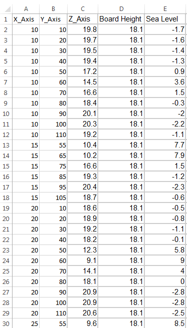Figure 3: The processed data ready to be imported into ArcMap and converted into a shapefile.

After correcting the data values, added the spreadsheet to an ArcMap document, and created an event layer of the points by right clicking and selecting "Add XY Data". Next, I exported the event layer to my geodatabase, where I saved it as a feature class. At this point, I opened model builder and ran 5 interpolation methods to generate surfaces from my feature class. 

IDW (Inverse Distance Weighted):

IDW estimates cell values by averaging the values of the 12 closest points to each cell. Points that are closer to the cell have greater weight on the interpolated value of the cell.  

Figure 4: This surface was interpolated using IDW.
This method produced good results where the 12 closest points had similar heights, like the plain to the upper right.

Kriging:

Kriging uses a two-step process to interpolate a surface. First, it selects a group of points and attempts to fit a model to the points in order to determine how much of an influence spatial autocorrelation plays in the model. After determining the influence of spatial autocorrelation, it uses the previously created model to weight values, and uses them to derive predictions for unmeasured locations.

Figure 5: This surface was interpolated using Kriging.

Natural Neighbors:

Natural Neighbor interpolation creates polygons around each of the given points, and interpolates the area between a query point and its nearest neighboring points by proportionally weighting their elevation values by how much their polygons overlap a polygon created around the query point. Points with larger amounts of overlap will have higher weights than points with smaller amounts of overlap, even if they are the same distance away (differentiating it from IDW). This method produces smooth areas everywhere except at the survey point locations where the terrain will be more sharply angled.

Figure 6: This surface was interpolated using Natural Neighbors.

Spline: 

Spline works by fitting the elevation points to mathematical functions so that the interpolated surface passes through every single data point, to minimize the overall curvature of the surface. Areas between survey points may be slightly more extreme than the surveyed values, so the surface will appear more smooth and rounded.

Figure 7: This surface was interpolated using Spline.

TIN (Triangular Irregular Network):

Unlike the previous raster-based interpolation methods, TIN is vector based. TIN takes input points and uses the Delaunay triangulation method to form a continuous, triangulated surface. Lines can be added to tell the TIN where drastic changes in elevation - like streams, roads, or ridge-lines - occur so it can enforce abrupt changes of elevations at those locations. Because the surface resolution of TIN is reliant on the point density, if areas with greater elevation change are sampled more densely, the TIN will calculate those areas with greater resolution, and more accurate results will be obtained.

Figure 8: This surface was interpolated using TIN.

Discussion:

IDW produced the least accurate interpolated surface overall. The results for IDW were skewed in areas where the 12 closest weighted points had extreme differences in their heights. In these situations, cells within a close proximity to a survey point were accurate to the surveyed elevation, but cells between sample points became extremely skewed as points with extremely different elevations started to become weighted evenly. This is extremely evident on the ridge, the valley, and the depression (Figure 9).

The TIN surface did well at maintaining the shape and accurate elevations for the hill and ridge-line (Figure 9). It also showed the elevation discontinuity between the plain and valley with the greatest clarity. Although its results were fairly accurate for those areas, the rest of the terrain suffered. TIN produced extremely inaccurate results in areas, like the valley, where its point spacing caused its triangles to be interpolating too large of areas (Figure 8). TIN would have generated a more accurate and aesthetically pleasing surface had we sampled areas of dramatic elevation with higher point density. We could've also recorded lines, to enforce breaks in the elevation for the bottom and edges of the valley, and on the ridge-line.

Natural Neighbors also performed well at interpolating most of the features. The bottom of the valley is shown as a continuous area of low elevation, as it was in the original terrain (Figure 10). When it comes to areas with great differences in elevation, it starts to suffer from the same problems as IDW. As the survey points remain with their original elevations, the areas between and around them are averaged. This caused the top of the hill and ridge, the bottom of the depression, and the area between the valley and the plain to all have unnecessarily jagged shapes at the locations of the survey points (Figures 9,10).

Spline created an aesthetically pleasing surface model who's only fault is its inaccuracy. Spline over-smoothed certain areas, like the edge of the valley and plain, so the canyon-like wall of the valley has been replaced with a gently rolling slope down to the valley floor (Figure 10). The valley floor also had some effects of being excessively smoothed, as its low area of continuous elevation has been replaced with a series of rounded kettle-holes (Figure 9). The ridge and hill were both rounded to the point that they no longer resemble the shape of the original terrain's features (Figure 10).

Kriging created the most accurate model overall. This was due to how it analyzed the trends of the data before interpolating. The ridge was interpolated as a continuous high region across the map with areas between the survey points having almost the same elevation as the points themselves (Figure 9). The valley was interpolated as a continuous region of low elevation, rather than a series of depressions, much like the original terrain (Figure 10). The hill and depression are accurate to their actual shape and size with the survey points adding to the shape, but not appearing pointedly out of place (Figures 9,10).

When we generated interpolated surfaces with our survey data from part 1, we realized that our consistent point density was limiting the accuracy of our interpolated surfaces in areas with dramatic elevation changes. The addition of the offset points aided the accuracy of the interpolation calculations dramatically in these areas. Unfortunately, as our landscape was almost completely eroded by rainfall between our first and second surveys, we were forced to reconstruct the landscape and perform a second complete survey, rather than just adding points at the offset locations. Using a laterally held measuring stick to find values along the X and Y axis rather than two strings caused the entire surveying process to be 15 minutes faster, even though 85 more points were recorded. When I first tried to bring the data from our first survey into ArcScene, it was incredibly skewed because the data for the X and Y axes and the Z axis were in different units. When conducting the second survey, I recorded the points in the same unit, which completely eliminated the problem.

Figure 9: Profile comparison of the the interpolation methods.

Figure 10: Comparison of: the original terrain to: A. Kriging, B. Spline, and C. Natural Neighbors

Conclusion:

The terrain surveying exercise was extremely eye-opening to how important point density is when attempting to interpolate surfaces from data points. In the past, I have generated TIN datasets from points collected with LiDAR, and a lack of point density has never been an issue, naturally I was caught off guard when our first TIN was horrendously inaccurate. After conducting the second survey, I believed my group had small enough point spacing to generate a fairly accurate TIN surface, but I was again wrong! This lab really stressed the importance of stratified data collection, as the balance between high data density and time spent surveying must both be considered.

If I were to perform another survey, I would do so using a Microsoft Kinect as a makeshift LiDAR sensor to generate a point cloud of the survey area. I would also use the old survey method to record and create several breaklines of key features: the edge of the depression, the crest of the ridge, the edges of the valley, the base of the valley, and the base of the hill. I would then convert the kinect points to a multipoint dataset, and create a TIN using the mulitpoints and the hard breaklines. Unfortunately, I didn't have access to a Kinect sensor when we conducted our second survey, otherwise I would've attempted to use it as a form of ground-truthing.

Assessment: http://psawallgeospatialfieldmethods.blogspot.com/2015/09/exercise-assessments.html

Sources:
http://desktop.arcgis.com/en/desktop/latest/tools/3d-analyst-toolbox/how-idw-works.htm
http://desktop.arcgis.com/en/desktop/latest/tools/3d-analyst-toolbox/how-kriging-works.htm
http://desktop.arcgis.com/en/desktop/latest/tools/3d-analyst-toolbox/how-natural-neighbor-works.htm
http://desktop.arcgis.com/en/desktop/latest/tools/3d-analyst-toolbox/how-spline-works.htm
http://desktop.arcgis.com/en/desktop/latest/manage-data/tin/fundamentals-of-creating-tins.htm

Exercise Assessments

Exercise 1:

Prior to this activity, I would rank myself as having some knowledge on this topic. 3
Following this activity, I would rank myself as having enough knowledge to teach someone else about the topic. 4
The hands-on approach to this activity greatly added to how much I was able to learn. 5

In order to make the activity better, I would find some way to preserve the landscapes throughout the week, so they can be fully intact for future activities.

Exercise 2:

Prior to this activity, how would you rank yourself in knowledge about the topic. 

3-Some knowledge
Following this activity, how would you rate the amount of knowledge you have on the topic 

4-I know enough to teach someone else
Did the hands-on approach to this activity add to how much you were able to learn

5-Strongly Agree
What types of learning strategies would you recommend to make the activity even better? 

I would recommend using either a Kinect sensor or photoscan to generate an accurate representation of the terrain surface to truly see where different interpolation methods produced errors.

Terrain Creation and Survey

Introduction:

We were tasked to create a landscape within a 1.26m x 1.19m wooden frame featuring: a plain, a mountain, a ridge, a valley, and a depression. After forming our landscape, we were to survey the surface of the landscape for future mapping purposes. We were to form our landscape on the sandy point bar of the Chippewa River underneath the UW-EC campus footbridge.

Methods:

Before shaping the terrain, we leveled the ground surface underneath the survey frame, in order to standardize the elevations for our survey. After the frame was leveled, we created a hill along the left side of the frame, a valley running from the top left to the bottom right, a ridge running parallel to the valley, a depression in the top right corner, and a plain in the lower left corner (Figures 4-5). Next, we put scotch tape over the edges of the frame and marked them with a pen at 10cm intervals from a point of origin on the inside edge of “1D” on the frame (Figures 1-3). The boards themselves were all the same length, but due to the frame’s design, the X-axis (from 1D to 1B) was 1.26m long, and the Y-axis (from 1D to 1C) was 1.19m long. We made a grid with a sampling interval of 1dm, making a 12 x 11 grid with 132 total points. We started our survey at (1,1) which we found by placing modifiable string gridlines 10cm from the origin point of the X and Y-axes. After the gridlines were in place and pulled taut, we recorded the distance from the gridlines to the ground surface using a meter stick and recorded them in centimeters to 1mm accuracy (Figures 6-8). We recorded the distances from the grid to the ground as Z-values in a Google drive spreadsheet. After scanning point (1,1,19.8), we scanned (1,2,19.8) and continued working our way up the Y-axis until reaching the top of the frame, at which point we moved to (2,1,19.3) and followed the same procedure. We continued in this fashion until the survey was completed. We decided to use the base of the boards as our sea level. The boards of the frame measured 18.1cm tall, so I created a calculated column in Excel to subtract the distance between the gridline and the ground from the frame height. This made a new column with the height above or below sea level.

Discussion/Conclusion:

Leveling the frame was incredibly helpful, as it allowed us to record the actual slope of the pre-existing plain, and the landscape as a whole. Choosing the base of the frame as “sea level” wasn’t the best practice as most of the plain and other features are below “sea level”. Measuring the distance below the gridlines allowed most areas to be measured with ease, as none of our features surpassed the frame height. The only area that caused difficulties was the middle of the frame between (5,5) and (8,7), as they caused a lot of movement in the arm of our ruler holder as he was surpassing the comfortable range of his reach. This area was also more difficult to survey because the distance from the ruler caused some issues with properly sighting the distances between the ruler and the gridlines. Upon conducting a little research into sampling methods, I learned that my group conducted our survey using “systematic sampling” and that this sampling method may have caused us to under-sample some areas and features that fell between the gridlines. To compensate for this under-sampling, we should have instead used the “stratified random sampling” method. In order to have used “stratified random sampling” we would have created a grid system, and sampled one random point from within each individual square of the grid, rather than just from their verticies.

Figure 1. Marking the X and Y axes on the leveled frame

Figure 2. Ensuring we have accurate measurements

Figure 3.

Figure 4. The origin point is in the lower right corner of this photograph.

Figure 5. The origin point is in the bottom of the frame.
Clockwise from the left: Depression, Ridge, Plain, Hill, and Valley

Figure 6. The grid set up to record (1,10) the origin is to the right.

Figure 7. Recording point (1, 10, 22.9)

Figure 8. Conducting the survey.

Sources: http://uts.cc.utexas.edu/~wd/courses/373F/notes/lec15sam.html